Creating Interactive Maps of Earthquakes in R
library(readr)
library(tidyverse)
library(leaflet)
library(knitr)
Maps are a meaningful and simple way of presenting data. There are many ways to create maps in R, but one of the best is the leaflet package because it allows you to make them interactive! Today, I wanted to walkthrough using it and a couple of its many features.
Disclaimer! This post is not an exercise in statistical inference but rather a proof of concept of how to use the leaflet package.
Before we start, a little background:
Leaflet is the leading open-source JavaScript library for mobile-friendly interactive maps. It’s used by industry leaders ranging from The Washington Post and NPR to Github and Facebook, as well as the National Park Service and the federal government. The leaflet package in R makes it easy to create maps with map tiles that can be annotated with markers, lines, and popups.
Features
As explained by its creators, the leaflet package in R has the following features:
- Interative panning/zooming
- Composing maps using combinations of:
- Map tiles
- Markers
- Polygons
- Lines
- Popups
- GeoJSON
- Creating maps right from RStudio or the R console
- Embedding maps in R Markdown documents and Shiny apps
- etc.
Here is an example of producing maps of earthquakes from 1965 to the present. I found data collected by the National Earthquake Information Center (NEIC) on Kaggle, which includes a record of the date, time, location, depth, magnitude, and source of every earthquake with a reported magnitude 5.5 or higher since 1965.
The entire process of making maps with leaflet boils down to 4 steps:
- Gather the data
- Create a map widget by calling
leaflet() - Add layers to the map by using layers (Ex:
addTiles,addMarkers,addPolygons) - Repeat step 3 as many times as desired
#Step 1
earthquakes <- read_csv("earthquakes.csv")
earthquakes$Date <- as.Date(earthquakes$Date, format = "%m/%d/%Y")
earthquakes$Year <- format(as.Date(earthquakes$Date, format = "%d/%m/%Y"),"%Y")
head(earthquakes) %>% kable()| Date | Time | Latitude | Longitude | Type | Depth | Depth Error | Depth Seismic Stations | Magnitude | Magnitude Type | Magnitude Error | Magnitude Seismic Stations | Azimuthal Gap | Horizontal Distance | Horizontal Error | Root Mean Square | ID | Source | Location Source | Magnitude Source | Status | Year |
|---|---|---|---|---|---|---|---|---|---|---|---|---|---|---|---|---|---|---|---|---|---|
| 1965-01-02 | 13:44:18 | 19.246 | 145.616 | Earthquake | 131.6 | NA | NA | 6.0 | MW | NA | NA | NA | NA | NA | NA | ISCGEM860706 | ISCGEM | ISCGEM | ISCGEM | Automatic | 1965 |
| 1965-01-04 | 11:29:49 | 1.863 | 127.352 | Earthquake | 80.0 | NA | NA | 5.8 | MW | NA | NA | NA | NA | NA | NA | ISCGEM860737 | ISCGEM | ISCGEM | ISCGEM | Automatic | 1965 |
| 1965-01-05 | 18:05:58 | -20.579 | -173.972 | Earthquake | 20.0 | NA | NA | 6.2 | MW | NA | NA | NA | NA | NA | NA | ISCGEM860762 | ISCGEM | ISCGEM | ISCGEM | Automatic | 1965 |
| 1965-01-08 | 18:49:43 | -59.076 | -23.557 | Earthquake | 15.0 | NA | NA | 5.8 | MW | NA | NA | NA | NA | NA | NA | ISCGEM860856 | ISCGEM | ISCGEM | ISCGEM | Automatic | 1965 |
| 1965-01-09 | 13:32:50 | 11.938 | 126.427 | Earthquake | 15.0 | NA | NA | 5.8 | MW | NA | NA | NA | NA | NA | NA | ISCGEM860890 | ISCGEM | ISCGEM | ISCGEM | Automatic | 1965 |
| 1965-01-10 | 13:36:32 | -13.405 | 166.629 | Earthquake | 35.0 | NA | NA | 6.7 | MW | NA | NA | NA | NA | NA | NA | ISCGEM860922 | ISCGEM | ISCGEM | ISCGEM | Automatic | 1965 |
On top of reading in the data, I went ahead and formatted the Date so that it is not a character, but instead a date. I also create a new variable with just the year so that we can look at the number of earthquakes by year.
Let’s start by creating a map that shows the earthquakes’ locations and magnitudes. I will do so by adding tiles, which basically create the map, followed by adding circles that are colored based on magnitude. We use the ifelse function to split the earthquakes into 4 ranges in terms of magnitude and assign a color to each of the ranges.
earthquakes %>%
  filter(Magnitude >= 7) %>%
  leaflet() %>% #Step 2
  #Step 3-4
  addTiles() %>%
  addCircles(~Longitude, ~Latitude, radius = 10, color = ~ifelse(Magnitude < 7.5, "green", ifelse(Magnitude < 8, "yellow", ifelse(Magnitude < 8.5, "blue", "red"))), label = ~as.character(paste("Earthquake Date: ", earthquakes$Date)))
The East coast of Asia and West coast the Americas seem most affected. The map has a little too much information, so it is hard to interpret much more at first glance. How about we find which year had the most earthqaukes? We will use ggplot2to plot the top 10 years with most earthquakes.
top_10 <- earthquakes %>%
  group_by(Year) %>%
  summarise(n=n()) %>%
  arrange(desc(n)) %>%
  head(10)
top_10 %>%
  ggplot(aes(x=reorder(Year,n), y=n)) +
  geom_bar(stat = "identity", fill = "blue") +
  labs(x="Year", y="Count", title = "Top 10 Years with Highest Earthquake Frequency") +
  coord_flip() +
  theme_bw() +
  theme(plot.title = element_text(hjust = 0.5))
The year with the most is 2011. (There seems to be a big difference between 2011 and 2007. I wonder why). As another exercise, we can map the location of the earthquakes in 2011. Once again, we will start by adding tiles and then circles. This time around I will keep all of points the same color.
earthquakes %>%
  filter(Year == 2011) %>%
  leaflet() %>% #Step 2
  #Step 3-4
  addTiles() %>%
  addCircles(~Longitude, ~Latitude, radius = 10, color = "blue")
Other useful features in addMarkers() are clustering and popups. Let’s try them out by building a map with the location of every earthquake grouped by region. One of the problems we ran into earlier was that we had a large number of markers in close proximity. We will use clusterOptions in addMarkers() to fix it.
earthquakes %>%
leaflet() %>% #Step 2
#Steps 3 and 4
addTiles() %>%
addMarkers(~Longitude, ~Latitude, clusterOptions = markerClusterOptions(maxClusterRadius=50),
popup = paste(earthquakes$Type,
"<br><strong>Magnitude: </strong>", earthquakes$Magnitude,
"<br><strong>Depth: </strong>", earthquakes$Depth,
"<br><strong>Date: </strong>", earthquakes$Date,
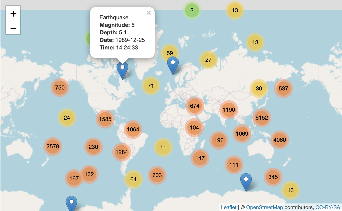
"<br><strong>Time: </strong>", earthquakes$Time))As you zoom in or pan, the clusters adjust. The other feature that I added was to have information in each marker. If you click on one of the markers, you see a popup with the type of disruption (there are 178 observations that are nuclear explosions and 1 burst rock), magnitude, depth, date, and time of day. I had to use some very simple HTML for the popup, which can be seen in the code above.
Here is an example of what happens if we click one:
If you want more information be sure to check out the RStudio leaflet webpage, which explains many more features that can be integrated into your maps.
As always, if you have a question or a suggestion related to the topic covered in this article, please feel free to contact me!