Investigating Chicago Traffic Crashes with RSocrata
library(tidyverse)
library(RSocrata)
library(knitr)
The incentive for this article was to try out the RSocrata package since it allows you to access a wealth of open data resources from governments, non-profits, and NGOs around the world. On top of that, it never hurts to practice using the tidyverse functions.
The dataset I will use shows information about each traffic crash on city streets within the City of Chicago limits and under the jurisdiction of Chicago Police Department.
We will download the last two years of data to explore. (Dont be alarmed if this next chunk of code takes a little longer to run. It is because we are scraping over 500,000 data points)
years_ago <- lubridate::today() - lubridate::years(2)
crash_url <- glue::glue("https://data.cityofchicago.org/Transportation/Traffic-Crashes-Crashes/85ca-t3if?$where=CRASH_DATE > '{years_ago}'")
crash_raw <- as_tibble(read.socrata(crash_url))
Here is a look at the dataset:
crash <- crash_raw %>%
  arrange(desc(crash_date)) %>%
  transmute(
    injuries = if_else(injuries_total > 0, "injuries", "none"),
    crash_date,
    crash_hour,
    report_type = if_else(report_type == "", "UNKNOWN", report_type),
    num_units,
    posted_speed_limit,
    weather_condition,
    lighting_condition,
    roadway_surface_cond,
    first_crash_type,
    trafficway_type,
    prim_contributory_cause,
    latitude, longitude
  ) %>%
  na.omit()

head(crash) %>% kable()| injuries | crash_date | crash_hour | report_type | num_units | posted_speed_limit | weather_condition | lighting_condition | roadway_surface_cond | first_crash_type | trafficway_type | prim_contributory_cause | latitude | longitude |
|---|---|---|---|---|---|---|---|---|---|---|---|---|---|
| none | 2021-06-03 01:38:00 | 1 | ON SCENE | 3 | 30 | CLEAR | DARKNESS, LIGHTED ROAD | UNKNOWN | PARKED MOTOR VEHICLE | ONE-WAY | UNABLE TO DETERMINE | 41.90705 | -87.75947 |
| none | 2021-06-03 01:20:00 | 1 | ON SCENE | 3 | 30 | CLEAR | DARKNESS, LIGHTED ROAD | DRY | PARKED MOTOR VEHICLE | NOT DIVIDED | UNABLE TO DETERMINE | 41.90159 | -87.76578 |
| none | 2021-06-03 00:50:00 | 0 | ON SCENE | 2 | 25 | CLEAR | DARKNESS, LIGHTED ROAD | DRY | ANGLE | T-INTERSECTION | DISREGARDING STOP SIGN | 41.88681 | -87.67694 |
| injuries | 2021-06-03 00:25:00 | 0 | ON SCENE | 1 | 30 | CLEAR | DARKNESS, LIGHTED ROAD | DRY | FIXED OBJECT | DIVIDED - W/MEDIAN (NOT RAISED) | PHYSICAL CONDITION OF DRIVER | 41.88621 | -87.74077 |
| none | 2021-06-03 00:10:00 | 0 | ON SCENE | 2 | 30 | CLEAR | DARKNESS | DRY | TURNING | NOT DIVIDED | UNABLE TO DETERMINE | 41.75073 | -87.70161 |
| injuries | 2021-06-03 00:01:00 | 0 | ON SCENE | 3 | 30 | CLEAR | DARKNESS, LIGHTED ROAD | DRY | ANGLE | FOUR WAY | DISREGARDING TRAFFIC SIGNALS | 41.87491 | -87.68394 |
The dataset has the date and time of crash, speed limit, weather condition, lighting condition, the condition of the road, cause, location, and whether there were injuries or not. Let’s see how the number of crashes has changed over time.
crash %>%
  mutate(crash_date = lubridate::floor_date(crash_date, unit = "week")) %>%
  count(crash_date, injuries) %>%
  filter(
    crash_date != last(crash_date),
    crash_date != first(crash_date)) %>%
  ggplot(aes(crash_date, n, color = injuries)) +
  geom_line(size = 1.5, alpha = 0.7) +
  scale_y_continuous(limits = (c(0, NA))) +
  labs(
    x = NULL, y = "Number of traffic crashes per week",
    color = "Injuries?"
  )
The first thing that stands out is the impact of the global pandemic. There was a significant drop in the number of crashes per week at the beginning of 2020. After the fall, the number of crashes with injuries rebounded, but still remains below its pre-pandemic levels.
Since we see such a change in crashes with injuries and a smaller impact on non-injury crashes, it might be interesting to see how the injury rate has changed over time.
crash %>%
  mutate(crash_date = lubridate:: floor_date(crash_date, unit = 'week')) %>%
  count(crash_date, injuries) %>%
  filter(
    crash_date != last(crash_date),
    crash_date != first(crash_date)) %>%
  group_by(crash_date) %>%
  mutate(percent_injury = n/sum(n)) %>%
  ungroup() %>%
  filter(injuries == 'injuries') %>%
  ggplot(aes(crash_date, percent_injury)) +
  geom_line(size=1.5, alpha=0.7, color = 'midnightblue') +
  scale_y_continuous(limits = c(0,NA), labels = scales::percent_format()) +
  labs(x=NULL, y='Percent of crashes that involve injuries')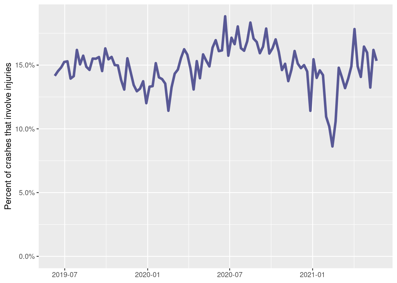
Suprisingly, the injury rate seemed to have increased during the pandemic. I was not expecting that. I wonder what caused that.
Have your parents ever told you to be careful when driving on the weekend because drivers are more reckless? Let’s see how true that is in this dataset. We will check how the injury rate changes over the course of the week.
crash %>%
  mutate(crash_date = lubridate::wday(crash_date, label = TRUE)) %>%
  count(crash_date, injuries) %>%
  group_by(injuries) %>%
  mutate(percent = n/sum(n)) %>%
  ungroup() %>%
  ggplot(aes(percent, crash_date, fill = injuries)) +
  geom_col(position = 'dodge', alpha=0.8) +
  scale_x_continuous(labels = scales::percent_format()) +
  labs(x='Percent of Crashes', y= NULL, fill = 'Injuries?') +
  coord_flip()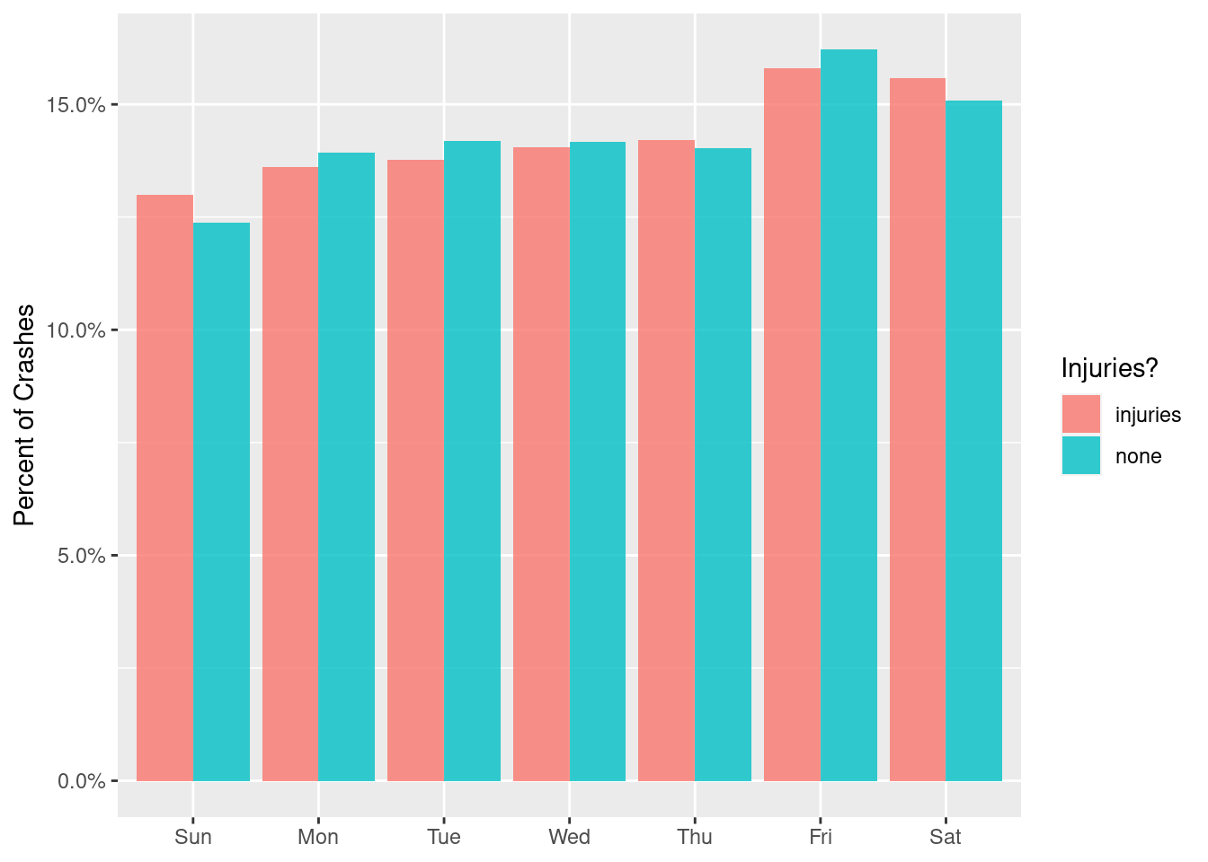
Friday and Saturday seem to have the highest injury rate, but the difference with the rest of the weekdays is not very large. Even though there might be some validity to my parents’ warning, the data does not reveal a significant relationship.
By the same token, my parents say that most crashes occur at night. Let’s check if this is reflected here.
crash %>%
  count(lighting_condition, injuries) %>%
  group_by(injuries) %>%
  mutate(percent = n/sum(n)) %>%
  ungroup() %>%
  ggplot(aes(percent, lighting_condition, fill = injuries)) +
  geom_col(position = 'dodge', alpha = 0.8) +
  scale_x_continuous(labels = scales::percent_format()) +
  labs(x='Percent of Crashes', y= NULL, fill = 'Injuries?')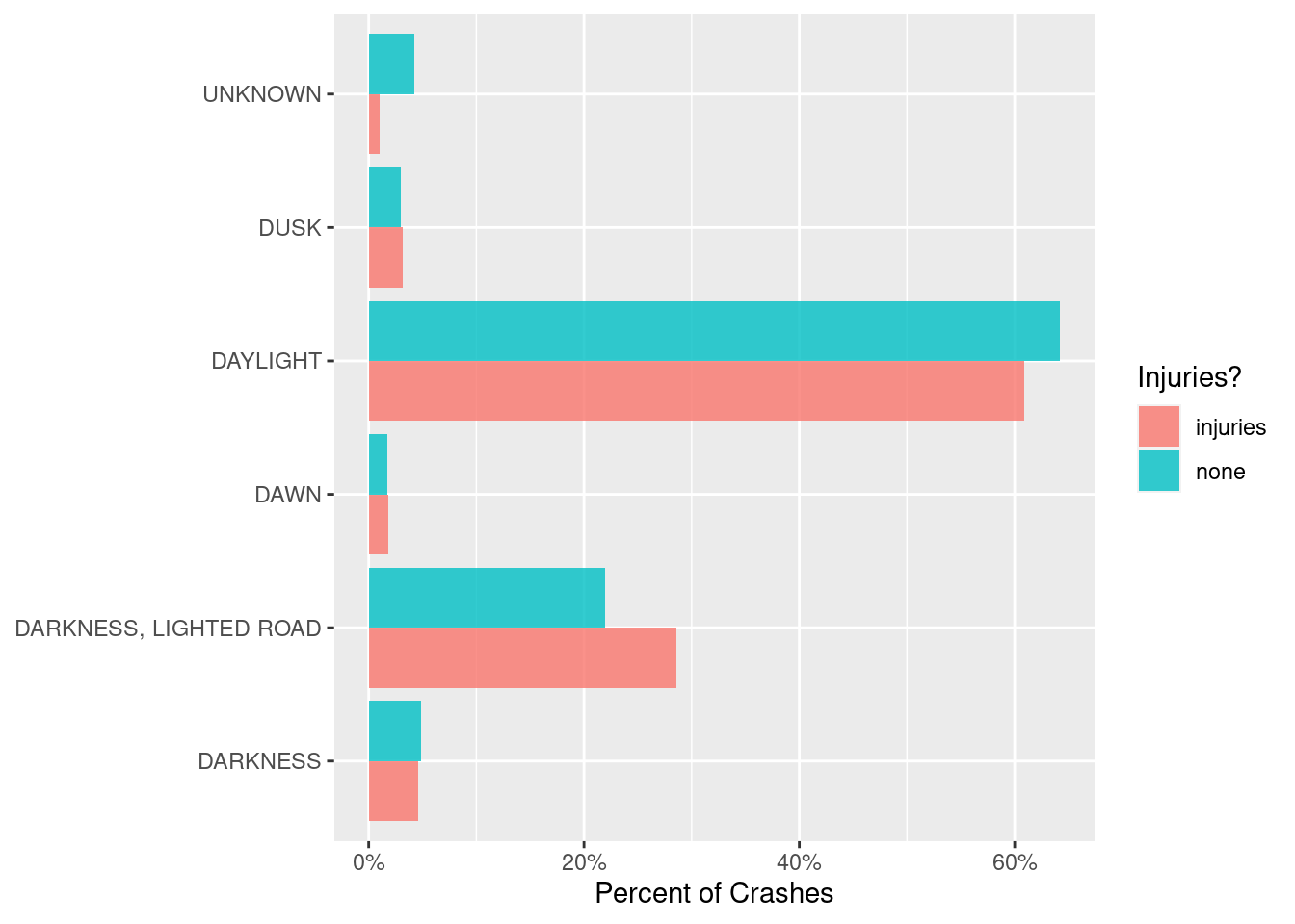
Predictably, the largest portion of crashes, both with and without injuries, take place during daylight. This makes sense since most car usage is during daylight.
Another thing we can look at is how injuries vary with the first crash type. Do certain type of crashes lead to more injuries?
crash %>%
  count(first_crash_type, injuries) %>%
  mutate(first_crash_type = fct_reorder(first_crash_type, n)) %>%
  group_by(injuries) %>%
  mutate(percent = n/sum(n)) %>%
  ungroup() %>%
  group_by(first_crash_type) %>%
  filter(sum(n)>1e4) %>%
  ungroup() %>%
  ggplot(aes(percent, first_crash_type, fill = injuries)) +
  geom_col(position = 'dodge', alpha = 0.8) +
  scale_x_continuous(labels = scales::percent_format()) +
  labs(x='Percent of Crashes', y=NULL, fill = 'Injuries?')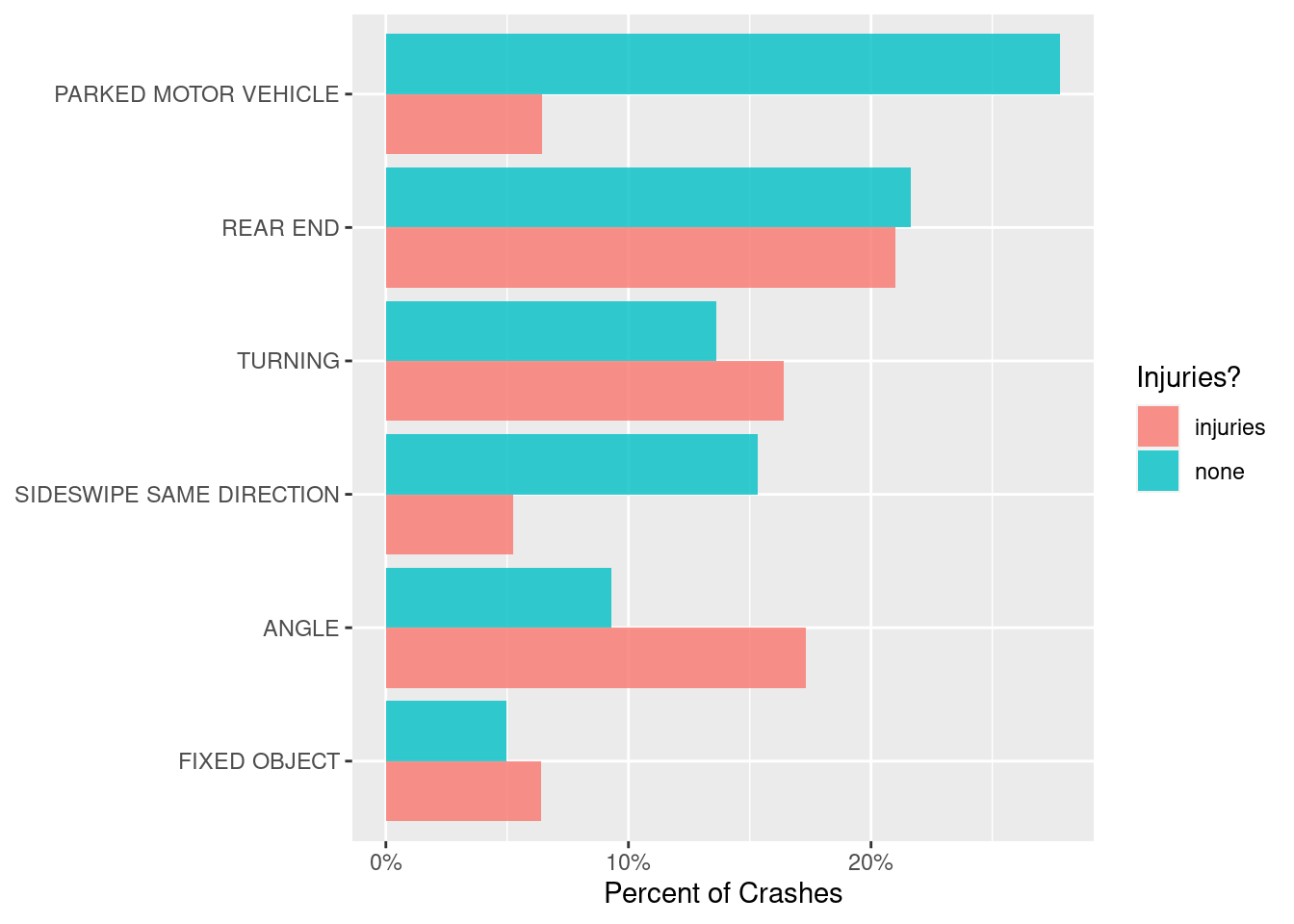
We can see that Rear End crashes are the most hurtful type, closely followed by turning and angle style crashes.
Now let’s look at where injuries are more common. Since we have both the longitude and latitude of each crash, we can create a map of the city and plot where injuries occur most.
crash %>%
  filter(latitude>0) %>%
  ggplot(aes(longitude, latitude, color = injuries)) +
  geom_point(size = 0.6, alpha = 0.5) +
  labs(color = NULL) +
  scale_color_manual(values = c("deeppink4", "gray80")) +
  coord_fixed() +
  theme(axis.title = element_blank())
The crashes with injuries seem to be dispered all throughout the city of Chicago.
As always, if you have a question or a suggestion related to the topic covered in this article, please feel free to contact me!